Excel 2000 Module 4
Formatting Worksheets
The
major benefits of using Microsoft Excel 2000 include the ability
to organize data in row-and-column format and then perform calculations
on specific rows, columns, and cells. Excel provides dozens
of ways to format labels and values in a worksheet to provide
a more attractive design and layout.
Start
<Excel>
Click <File>, <New>
Click <Sheet1>
Rename <Sheet1>
to <M4Ex>
Practice M4Ex
Using AutoFormat
With the AutoFormat feature, you can format the data in your worksheets using a professionally designed template.
Select Range A1:F8
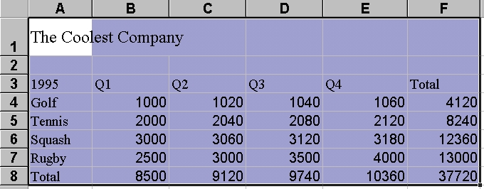
Click <Format> <AutoFormat>
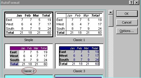
Select Classic 2 format Click <OK>


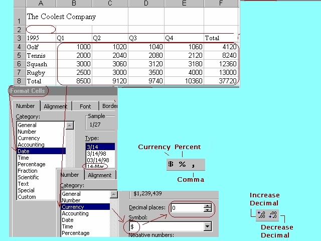
Formatting Numbers
Most of the data that you use in Excel is numeric. You can select one of Excel's options for formatting numbers. These options automatically insert and delete symbols and digits to reflect the format you choose.
By default, all data you enter is formatted with the General option, which shows the data exactly as you enter it.
You can choose from the following formats, organiszed by category :
General, Number, Currency,
Accounting, Date, Time,
Percentage, Fraction, Scientific,
Text, Special, Custom.
Click Cell A2
Use Today Function to enter the date
Format the date to dd/mm
Click <Format> <Cells>
Click <Number> tab Click <Date>
Select Type list Click <OK>
Select Range B4:F8
Click <Format> <Cells>
Click <Number> tab Click <Currency><$>
Click Decimal places down arrow
Select <0> Click <OK>
Alternatively

Click <$> button Click <,> button
Click <Decrease Decimal> button
Aligning Cell Contents
You can change the alignment relative to the edges of the cells. You can align horizontally or vertically with the option of the orientation in degrees.
Select Range A4:A8
Click <Format> <Cells>
Click <Alignment> tab
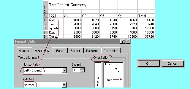
Select <Horizontal> arrow <Left (indent)>
Select <Vertical> arrow <Bottom>


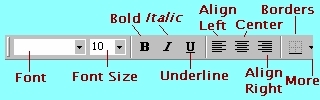
Formatting Text
You can change the font and font size for selected headings, labels, and values. A font is the general appearance of text, numbers, and other character symbils. Excel's default font is 10-point Arial. A point is 1/72 inch. So a 10 point font means about 1/6 inch high. The Font tab of the Format Cells dialog box contains options to change the font, the style and the point size of a cell entry.
Select Cell A2 (Today Date)
Click <Bold> button
Select Range A3:F3
Click <Center> Click <Bold>
Right Click, Select <Format Cells>
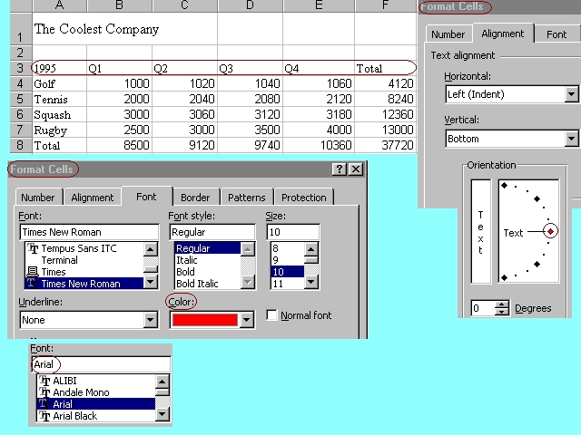
Click <Font> tab Select Font style list
Click <Arial>
Select Size list Click <12>
Click <Color> Select Red Click <OK>
Select Range A4:A8
Click <Bold> button
Right Click, Select <Format Cells>
Click <Alignment> tab
Select <left (Indent)> list
Type 1 at Indent box Click <OK>
Adding Borders
Adding borders to a cell or a range of cells can enhance the visual appeal of your worksheet, make it easire to read, and highligh particular data. You can put a border around the cell, a range of cells, or an entire worksheet.
Select Range B8:F8
Click <Border> button
Click <Thick Outline> button
A menu of border line styles and locations
Select Range A3:E3
Right Click, Select <Format Cells>
Click <Border> tab
Select <second line (right)> Line Style list
Click Blue
Click <Border> section to apply on
selected lines which is below only
Click <OK>

Adding Shading
You can add shading and patterns to a cell or a range of cells to set off the selection. Shading can be a shade of gray or a colour.
Select Range B8:F8
Click <Format> <Cells>
Click <Patterns> tab Click Yellow

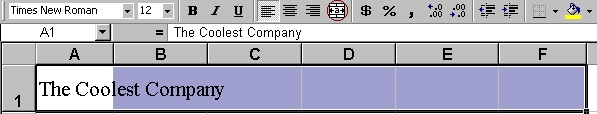
Merging Cells
Merging cells combines two or more cells into a single cell so that the text or value within the cell can be formatted more easily.
Select Range A1:F1
Click <Merge And Center>
Select Range A1:F1
Click <Format> <Cells>
Click Horizontal list Click <Centre>
Click Vertical list Click <Centre>
Select <Wrap Text> at the Text control
Select <Merge Cells> at the Text control
Click <OK>
Creating and Applying Conditional Formats
You can control how data appears in Excel worksheets by applying conditional formats, which are rules you create to determine how data appears depending on the value of the cell, e.g. set any numeric entry betwen 1500 and 2500 appears in Green.
Select Range B4:E4
Click <Format> <Conditional Formatting>
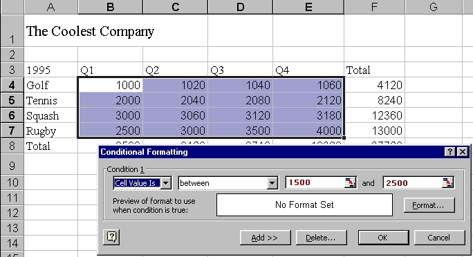
Click <between>
Type 1500 at the far left side
Type 2500 at the far right side
Click <OK>
The minimum and maximum value for the condition is set.
Click <Format> button
Click <Color> arrow for Green
Click <Bold> for Font Style list
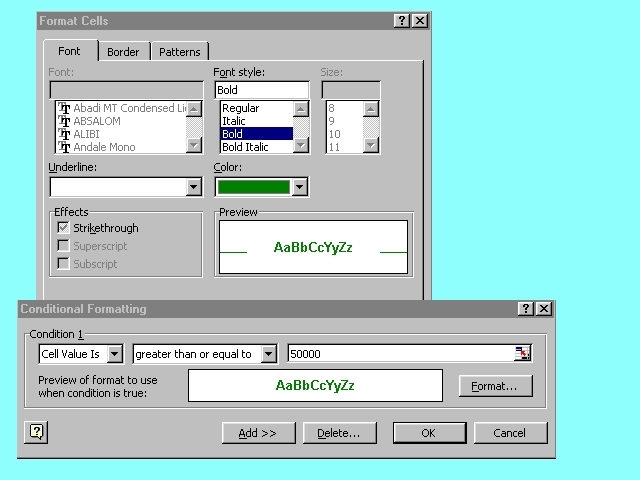
Click <OK>
Click <File> <Save>
Click <File> <Close>


Practice Exercise 1 : M4: Page 13
Click <Sheet2>
Rename <Sheet2>
to <M4Ex1>
Click
<File>
<Save>
Click <File> <Close>
Click <File> <Exit>
Practice Exercise 2
<New>
Workbook
Click
<File>
<Save As>
Excel2000
Project 1
at
<My Document>
<Save>
Practise
International
Sales for international currency formatting,
borders and shading.
Click
<File>
<Save>
Click <File> <Close>
Click <File> <Exit>
 Edwin
Koh : We
completed on the New
Knowledge and Skills in
Edwin
Koh : We
completed on the New
Knowledge and Skills in
Excel
2000 Module 4.